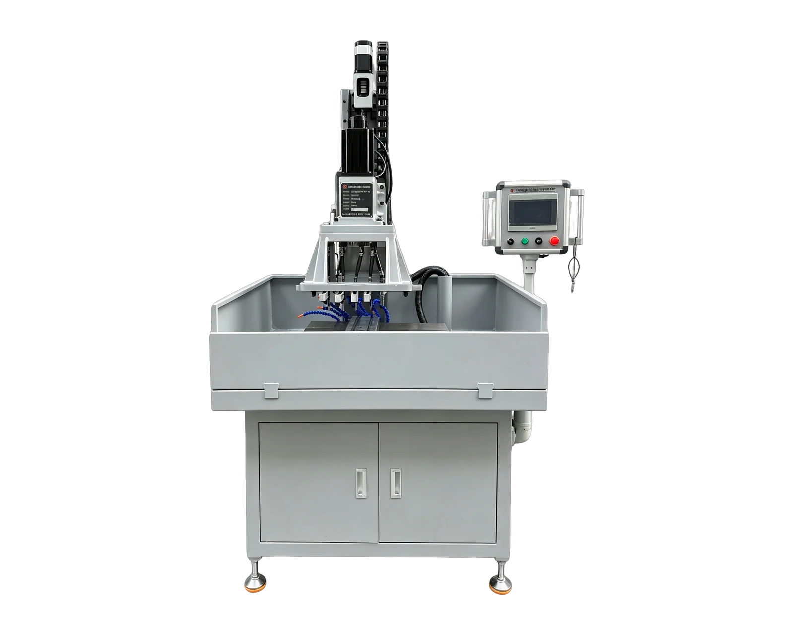
Explore equipment for your inquiry
Dual-Servo Multi-Spindle Drilling & Tapping Machine →Review the published specifications and configuration options against your part drawing before requesting a quote.
Define the period and what counts as a good part
Choose the same output specification, inspection boundary and analysis period for both routes. Here the period is one year and all amounts are illustrative US dollars. Volume Q is accepted parts per year, not spindle cycles or pieces started. A route that produces the wrong features cannot become a valid alternative merely because its estimated cost is low.
The SBA's break-even guidance distinguishes fixed and variable costs for a sales calculation. The model below instead equates the costs of two manufacturing routes. It uses an explicit algebraic comparison, with no selling-price assumption. Have your finance owner define annual fixed costs consistently: do not put the full purchase payment into one route and only annual depreciation into the other. Sunk spending and recoverable future spending should remain distinguishable.
Calculate the crossover from the cost difference
Let F_A and F_B be annual fixed costs for existing route A and dedicated route B. Let v_A and v_B be variable US dollars per good part. Then C_A = F_A + v_A × Q and C_B = F_B + v_B × Q. Setting C_A = C_B gives Q* = (F_B − F_A) ÷ (v_A − v_B), when the denominator is nonzero.
For the common case F_B > F_A and v_A > v_B, route B costs less above Q*. If B has no unit-cost saving, higher volume cannot offset its extra fixed cost in this model. If one route has both lower fixed and lower variable cost, there is no positive crossover in favor of the other. Capacity limits and changes in staffing can also invalidate a single straight-line comparison.
Reproduce this hypothetical one-year example
Assume F_A = US$6,000/year, F_B = US$18,000/year, v_A = US$0.80/good part and v_B = US$0.40/good part. The extra fixed cost is US$12,000/year and the unit saving is US$0.40. Therefore Q* = 12,000 ÷ 0.40 = 30,000 good parts/year. At that output each route totals US$30,000/year: 6,000 + 0.80 × 30,000 equals 18,000 + 0.40 × 30,000.
Every amount in this example is invented for arithmetic, not a BINSING price, performance estimate or customer result. The table changes one assumption at a time. The last column is C_A minus C_B at 40,000 good parts/year; a negative value means the dedicated route costs more under that scenario.
Replace each assumption with evidence before deciding
Use representative trial observations and actual purchasing records for variable costs. Account for accepted output, tool consumption and genuinely volume-dependent activities. If an operator remains employed for the same paid shift, fewer seconds of attendance do not automatically create an equal cash saving. Treat redeployed capacity separately unless the comparison explicitly values it. Do not charge a salaried operator once in annual fixed costs and again in a per-part allowance.
Check whether projected demand can actually use the capacity and whether the route can supply that demand after planned interruptions. Additional shifts, fixtures or maintenance may introduce cost steps. Recalculate by range when they do. For a capital approval, extend the analysis to the company's chosen cash-flow, financing, tax and residual-value treatment. This one-year screening model only answers where two stated annual cost lines intersect.